42 how to add data labels chart element in excel
Waterfall Chart in Excel - Easiest method to build. - XelPlus Just right mouse click on any series and go to the Change Series Chart Type… From the Change Series Chart Type… options, find the Data Label Position Series and change it to a Scatter Plot. Now things look better again. Click on the Data Label Position Series or select it from the Series Options. Activate data labels and position these on top. Broken Y Axis in an Excel Chart - Peltier Tech 11/18/2011 · Add the secondary horizontal axis. Excel by default puts it at the top of the chart, and the bars hang from the axis down to the values they represent. ... No need to dwell on it in the chart. The gap in the data or axis labels indicate that there is missing data. An actual break in the axis does so as well, but if this is used to remove the ...
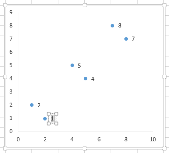
How to Create a Quadrant Chart in Excel – Automate Excel Step #9: Add the default data labels. We’re almost done. It’s time to add the data labels to the chart. Right-click any data marker (any dot) and click “Add Data Labels.” Step #10: Replace the default data labels with custom ones. Link the dots on the chart to the corresponding marketing channel names.

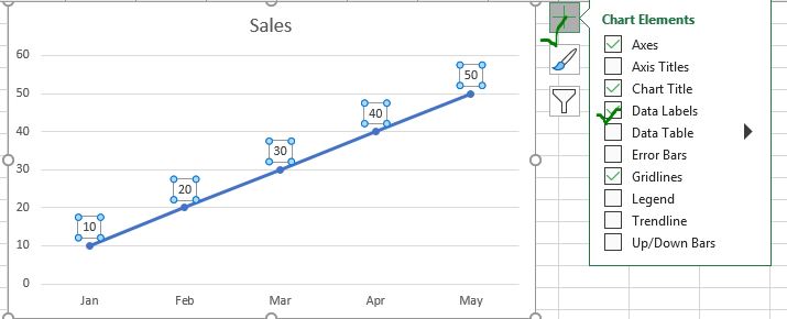
How to add data labels chart element in excel
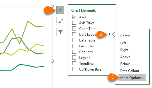
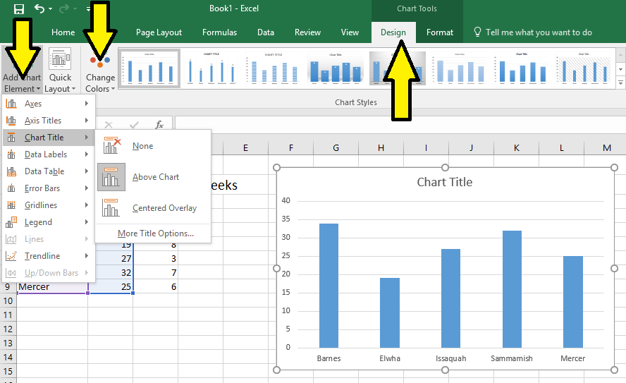
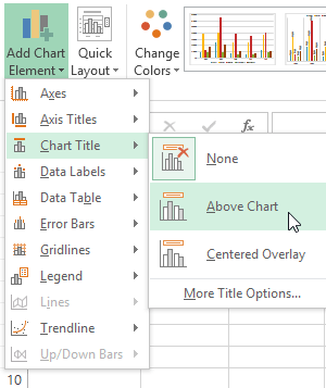
Change the format of data labels in a chart To get there, after adding your data labels, select the data label to format, and then click Chart Elements > Data Labels > More Options. To go to the appropriate area, click one of the four icons ( Fill & Line , Effects , Size & Properties ( Layout & Properties in Outlook or Word), or Label Options ) shown here. How to Make a PIE Chart in Excel (Easy Step-by-Step Guide) Related tutorial: How to Copy Chart (Graph) Format in Excel Formatting the Data Labels. Adding the data labels to a Pie chart is super easy. Right-click on any of the slices and then click on Add Data Labels. As soon as you do this. data labels would be added to each slice of the Pie chart. How to Create a Graph in Excel: 12 Steps (with Pictures ... - wikiHow 5/31/2022 · Add a title to the graph. Double-click the "Chart Title" text at the top of the chart, then delete the "Chart Title" text, replace it with your own, and click a blank space on the graph. On a Mac, you'll instead click the Design tab, click Add Chart Element, select Chart Title, click a location, and type in the graph's title.
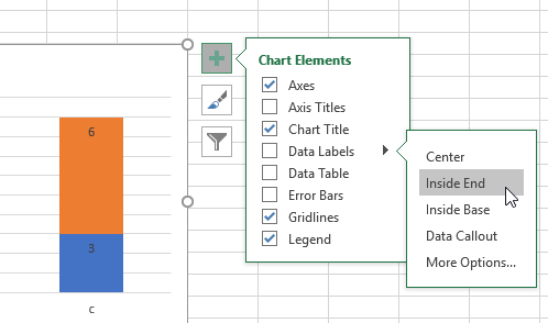
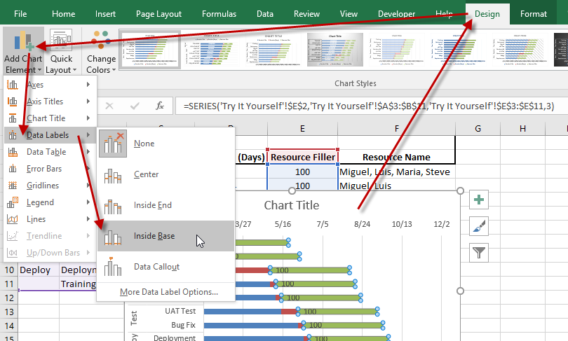
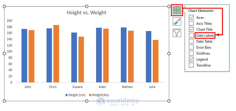
How to add data labels chart element in excel. Excel add-in tutorial - Office Add-ins | Microsoft Learn 9/13/2022 · To test your add-in in Excel on the web, run the following command in the root directory of your project. ... The labels on the data points across the bottom are in the sort order of the chart; that is, merchant names in reverse alphabetical order. Freeze a table header. ... Locate the element for the create-chart button, and add the ... Add or remove data labels in a chart - support.microsoft.com Depending on what you want to highlight on a chart, you can add labels to one series, all the series (the whole chart), or one data point. Add data labels. You can add data labels to show the data point values from the Excel sheet in the chart. This step applies to Word for Mac only: On the View menu, click Print Layout. How to Insert Axis Labels In An Excel Chart | Excelchat How to add vertical axis labels in Excel 2016/2013. We will again click on the chart to turn on the Chart Design tab . We will go to Chart Design and select Add Chart Element; Figure 6 – Insert axis labels in Excel . In the drop-down menu, we will click on Axis Titles, and subsequently, select Primary vertical . Figure 7 – Edit vertical ... How to Add Percentages to Excel Bar Chart – Excel Tutorial Once we do this we will click on our created Chart, then go to Chart Design >> Add Chart Element >> Data Labels >> Inside Base: Our chart will look like this: To lose the colors that we have on points percentage and to lose it in the title we will simply click anywhere on the small orange bars and then go to Format >> Shape Styles >> Shape Fill ...
How to Create a Graph in Excel: 12 Steps (with Pictures ... - wikiHow 5/31/2022 · Add a title to the graph. Double-click the "Chart Title" text at the top of the chart, then delete the "Chart Title" text, replace it with your own, and click a blank space on the graph. On a Mac, you'll instead click the Design tab, click Add Chart Element, select Chart Title, click a location, and type in the graph's title. How to Make a PIE Chart in Excel (Easy Step-by-Step Guide) Related tutorial: How to Copy Chart (Graph) Format in Excel Formatting the Data Labels. Adding the data labels to a Pie chart is super easy. Right-click on any of the slices and then click on Add Data Labels. As soon as you do this. data labels would be added to each slice of the Pie chart. Change the format of data labels in a chart To get there, after adding your data labels, select the data label to format, and then click Chart Elements > Data Labels > More Options. To go to the appropriate area, click one of the four icons ( Fill & Line , Effects , Size & Properties ( Layout & Properties in Outlook or Word), or Label Options ) shown here.
Quick Tip: Excel 2013 offers flexible data labels | TechRepublic

Apply Custom Data Labels to Charted Points - Peltier Tech

how to add data labels into Excel graphs — storytelling with data

Adding rich data labels to charts in Excel 2013 | Microsoft ...

Change the format of data labels in a chart
Dynamically Label Excel Chart Series Lines • My Online ...

Enable or Disable Excel Data Labels at the click of a button ...

Change the format of data labels in a chart
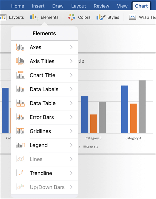
Modify charts in Office on mobile
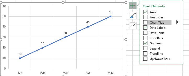
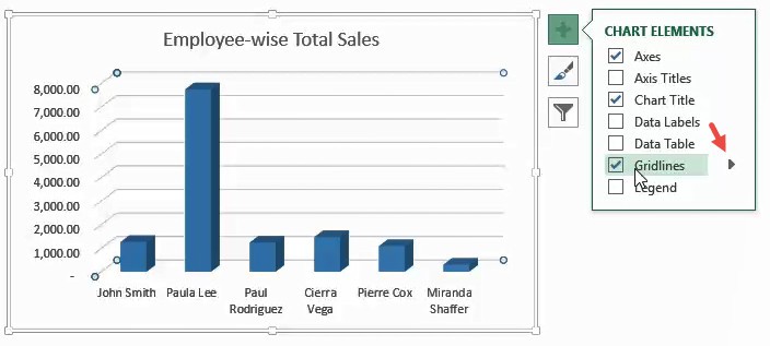
How to Add and Remove Chart Elements in Excel
Format Data Label: Label Position - Microsoft Community

How to Make a Pie Chart in Excel - All Things How

How to add axis titles in excel chart | WPS Office Academy
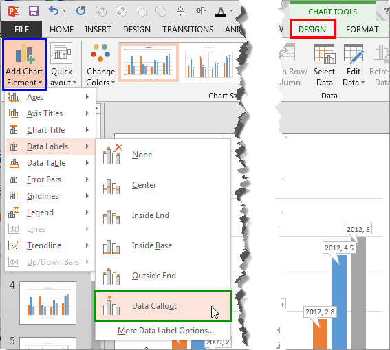
Callout Data Labels for Charts in PowerPoint 2013 for Windows
Graphing with Excel - BIOLOGY FOR LIFE
How to Add Gridlines in a Chart in Excel? 2 Easy Ways ...
Apply Custom Data Labels to Charted Points - Peltier Tech

Adding rich data labels to charts in Excel 2013 | Microsoft ...
Excel 2016 Gantt Chart Add Data Labels - Excel Dashboard ...

Add or remove data labels in a chart

how to add data labels into Excel graphs — storytelling with data
Excel 2013: Charts

How to insert data labels to a Pie chart in Excel 2013

How to add or move data labels in Excel chart?

Move and Align Chart Titles, Labels, Legends with the Arrow ...

CIS Ch3 Excel Flashcards | Quizlet
How to Add Data Labels in Excel (2 Handy Ways) - ExcelDemy

How to Add Total Data Labels to the Excel Stacked Bar Chart ...
How to Add Data Labels to a Chart - ExcelNotes

Custom data labels in a chart
How to Add and Remove Chart Elements in Excel

How to Add Data Labels to an Excel 2010 Chart - dummies

Chart axes, legend, data labels, trendline in Excel - Tech Funda

Pie Chart – Excel Tutorial

Display Customized Data Labels on Charts & Graphs

microsoft excel - Adding data label only to the last value ...
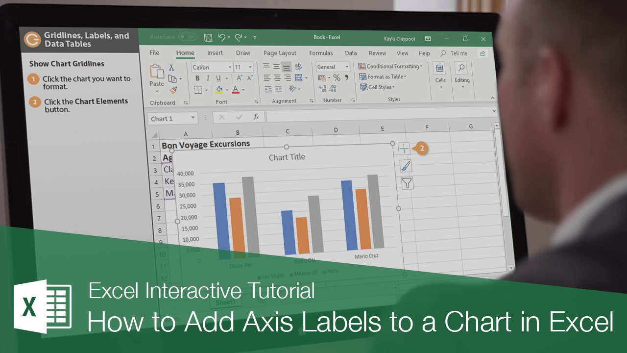
How to Add Axis Labels to a Chart in Excel | CustomGuide
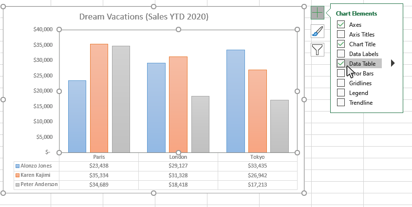
How to Add Data Tables to a Chart in Excel - Business ...

Add or remove data labels in a chart

Adding rich data labels to charts in Excel 2013 | Microsoft ...

Improve your X Y Scatter Chart with custom data labels

How to Add Data Labels to your Excel Chart in Excel 2013
Post a Comment for "42 how to add data labels chart element in excel"