44 multiple data labels excel pie chart
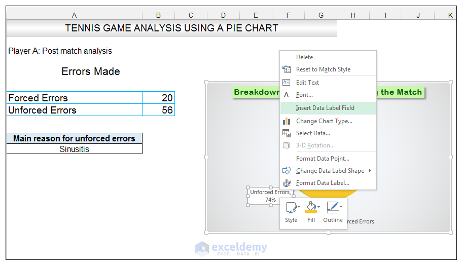
Add data labels and callouts to charts in Excel 365 | EasyTweaks.com Step #1: After generating the chart in Excel, right-click anywhere within the chart and select Add labels . Note that you can also select the very handy option of Adding data Callouts. Step #2: When you select the "Add Labels" option, all the different portions of the chart will automatically take on the corresponding values in the table ... Creating Pie Chart and Adding/Formatting Data Labels (Excel) Creating Pie Chart and Adding/Formatting Data Labels (Excel) Creating Pie Chart and Adding/Formatting Data Labels (Excel)
How to Create Multi-Category Charts in Excel? - GeeksforGeeks Implementation : Step 1: Insert the data into the cells in Excel. Now select all the data by dragging and then go to "Insert" and select "Insert Column or Bar Chart". A pop-down menu having 2-D and 3-D bars will occur and select "vertical bar" from it. Select the cell -> Insert -> Chart Groups -> 2-D Column.
Multiple data labels excel pie chart
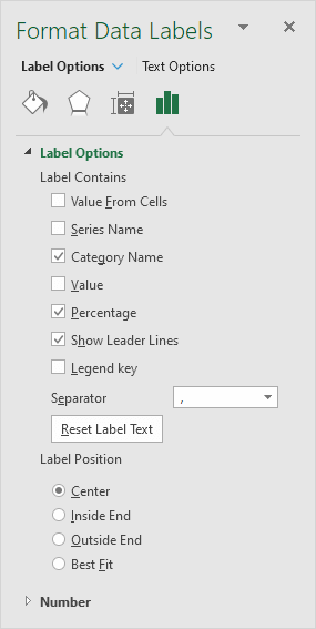
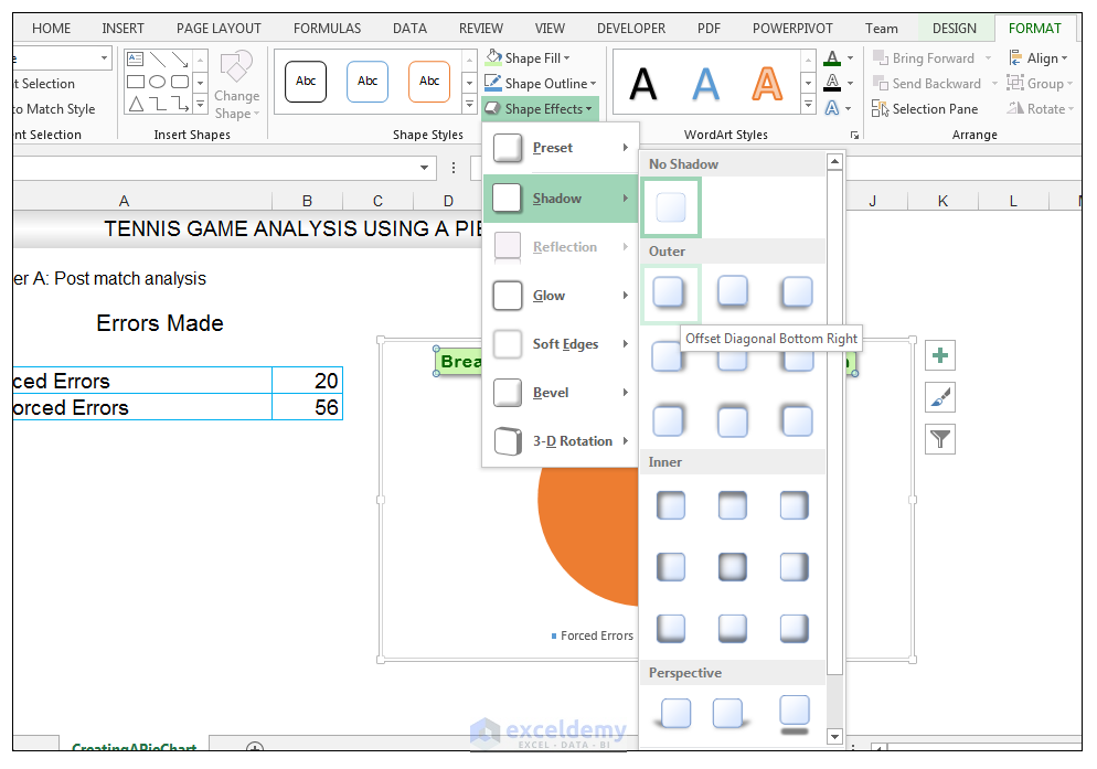
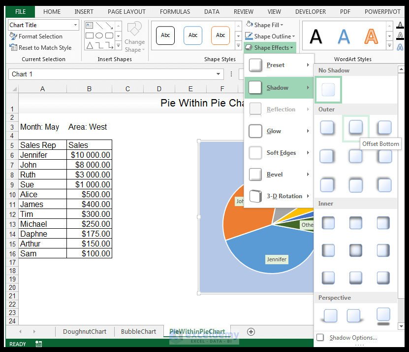
Change the format of data labels in a chart To get there, after adding your data labels, select the data label to format, and then click Chart Elements > Data Labels > More Options. To go to the appropriate area, click one of the four icons ( Fill & Line , Effects , Size & Properties ( Layout & Properties in Outlook or Word), or Label Options ) shown here. Create a multi-level category chart in Excel - ExtendOffice 2. Select the data range, click Insert > Insert Column or Bar Chart > Clustered Bar.. 3. Drag the chart border to enlarge the chart area. See the below demo. 4. Right click the bar and select Format Data Series from the right-clicking menu to open the Format Data Series pane.. Tips: You can also double click any of the bars to open the Format Data Series pane. Multiple data labels (in separate locations on chart) Running Excel 2010 2D pie chart I currently have a pie chart that has one data label already set. The Pie chart has the name of the category and value as data labels on the outside of the graph. I now need to add the percentage of the section on the INSIDE of the graph, centered within the pie section.
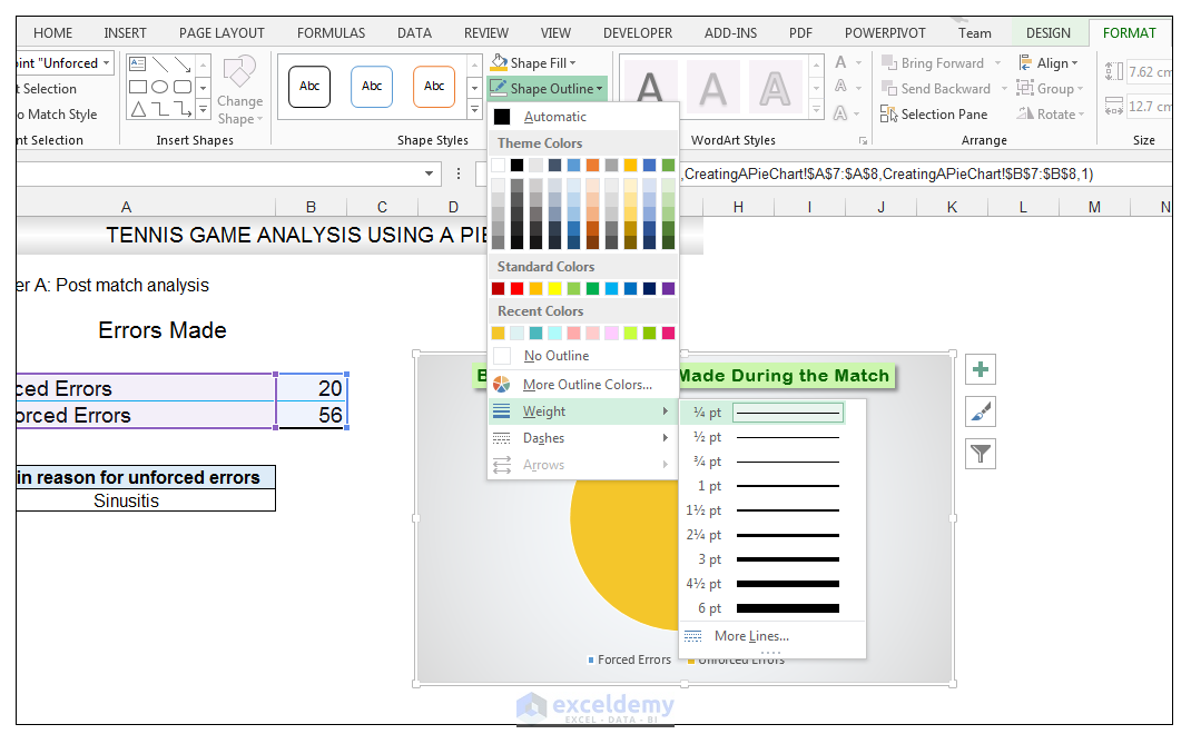
Multiple data labels excel pie chart. Power BI Pie Chart - Complete Tutorial - EnjoySharePoint 5.6.2021 · Power BI Pie chart is very useful to visualize the high-level data. It is a circular statistical format that represents the size of the item in one data series. The data points on a Pie chart present as a percentage of the whole pie. The total value of the Pie chart is 100%. The formula of Pie chart =( given data / total data)*360 › data-series-data-points-dataUnderstanding Excel Chart Data Series, Data Points, and Data ... Sep 19, 2020 · When multiple data series are plotted in one chart, each data series is identified by a unique color or shading pattern. Not all graphs include groups of related data or data series. In column or bar charts, if multiple columns or bars are the same color or have the same picture (in the case of a pictograph ), they comprise a single data series. How to Create a Pie Chart in Excel - Smartsheet Enter data into Excel with the desired numerical values at the end of the list. Create a Pie of Pie chart. Double-click the primary chart to open the Format Data Series window. Click Options and adjust the value for Second plot contains the last to match the number of categories you want in the "other" category. How to Make a Pie Chart in Excel & Add Rich Data Labels to The Chart! Creating and formatting the Pie Chart. 1) Select the data. 2) Go to Insert> Charts> click on the drop-down arrow next to Pie Chart and under 2-D Pie, select the Pie Chart, shown below. 3) Chang the chart title to Breakdown of Errors Made During the Match, by clicking on it and typing the new title.
› documents › excelHow to display leader lines in pie chart in Excel? To display leader lines in pie chart, you just need to check an option then drag the labels out. 1. Click at the chart, and right click to select Format Data Labels from context menu. 2. In the popping Format Data Labels dialog/pane, check Show Leader Lines in the Label Options section. See screenshot: 3. Close the dialog, now you can see some ... › office-addins-blog › 2015/11/05How to create a chart in Excel from multiple sheets - Ablebits Nov 05, 2015 · Supposing you have a few worksheets with revenue data for different years and you want to make a chart based on those data to visualize the general trend. 1. Create a chart based on your first sheet. Open your first Excel worksheet, select the data you want to plot in the chart, go to the Insert tab > Charts group, and choose the chart type you ... Solved: Show multiple data lables on a chart - Power BI I know they can be viewed as tool tips, but this is not sufficient for my needs. Many of my charts are copied to presentations and this added data is necessary for the end users. Solved! Go to Solution. 09-08-2017 12:54 AM. You can set Label Style as All detail labels within the pie chart: Formatting data labels and printing pie charts on Excel for Mac 2019 ... Work around: Select the area of the chart - by selecting the cells behind where the chart is sitting > Print area> Select print area>File > print>then set print perameters (paper size, fit to page etc.) > Print. This worked. 2. When formatting data labels on an extended bar of pie chart: Excel does not allow me to:
excelunlocked.com › pie-of-pie-chart-in-excelPie of Pie Chart in Excel - Inserting, Customizing - Excel ... Jan 03, 2022 · In the above example, there were a total of 6 data points. The Parent Pie chart represents three of them i.e Facebook, Youtube, and Instagram while the fourth data point named “Other” splits into a subset Pie chart that represents the rest of the three data points i.e Zee, Linkedin, and Hotstar. Plot Multiple Data Sets on the Same Chart in Excel Follow the below steps to implement the same: Step 1: Insert the data in the cells. After insertion, select the rows and columns by dragging the cursor. Step 2: Now click on Insert Tab from the top of the Excel window and then select Insert Line or Area Chart. From the pop-down menu select the first "2-D Line". Adding data labels to a pie chart - Excel General - OzGrid Excel General. Adding data labels to a pie chart. Laplacian; Feb 24th 2005 ... Adding data labels to a pie chart. Instead of HasDataLabels try ApplyDataLabels, HasDataLabels is not a property of a chart. ... I tried recording multiple macros (create the chart from scratch, modify a created chart, etc.) and still nothing about labels. The macros ... Create two data labels in pie chart? | MrExcel Message Board The boss wants an icon in each data label of a 6-slice pie chart. I can insert the image into the label but it often covers the text and value. Can I create a label for text/value and a second for the image? I can't put any of these values into the pie slice because some of the slices are quite small (<5%) and the data or image are not ...
How to Make a Pie Chart in Excel & Add Rich Data Labels to The Chart!
Add or remove data labels in a chart - support.microsoft.com On the Design tab, in the Chart Layouts group, click Add Chart Element, choose Data Labels, and then click None. Click a data label one time to select all data labels in a data series or two times to select just one data label that you want to delete, and then press DELETE. Right-click a data label, and then click Delete.

r - Pie chart with multiple tags/info in ggplot2 - Stack Overflow
How to Create and Format a Pie Chart in Excel - Lifewire To create a pie chart, highlight the data in cells A3 to B6 and follow these directions: On the ribbon, go to the Insert tab. Select Insert Pie Chart to display the available pie chart types. Hover over a chart type to read a description of the chart and to preview the pie chart. Choose a chart type.

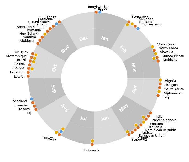
Nested donut chart (also known as Multi-level doughnut chart, Multi-series doughnut chart ...
Pie Chart in Excel | How to Create Pie Chart - EDUCBA Step 1: Select the data to go to Insert, click on PIE, and select 3-D pie chart. Step 2: Now, it instantly creates the 3-D pie chart for you. Step 3: Right-click on the pie and select Add Data Labels. This will add all the values we are showing on the slices of the pie.
How to Make a Pie Chart in Excel & Add Rich Data Labels to The Chart!
Multiple Data Labels on a Pie Chart - MrExcel Message Board Hello All, So I have a table with 8 rows and 3 columns. This table includes: Column 1 - shipment name. Column 2 - shipment cost. Column 3 - shipment weight. I have created a pie chart from this table, which covers the first two columns. Displayed next to each slice is a label with the shipment name, shipment cost, and percent share of the pie.

How to Make a Pie Chart in Excel & Add Rich Data Labels to The Chart!
Everything You Need to Know About Pie Chart in Excel How to Make a Pie Chart in Excel. Start with selecting your data in Excel. If you include data labels in your selection, Excel will automatically assign them to each column and generate the chart. Go to the INSERT tab in the Ribbon and click on the Pie Chart icon to see the pie chart types. Click on the desired chart to insert.
Create a Pie Chart in Excel - Easy Excel Tutorial
Create a Pie Chart in Excel - Easy Steps / Become a Pro 6. Create the pie chart (repeat steps 2-3). 7. Click the legend at the bottom and press Delete. 8. Select the pie chart. 9. Click the + button on the right side of the chart and click the check box next to Data Labels. 10. Click the paintbrush icon on the right side of the chart and change the color scheme of the pie chart. Result: 11.

How to Make a Pie Chart in Excel & Add Rich Data Labels to The Chart!
Excel Pie Chart Multiple Labels | Daily Catalog Add or remove data labels in a chart. Preview. 6 hours ago On the Design tab, in the Chart Layouts group, click Add Chart Element, choose Data Labels, and then click None.Click a data label one time to select all data labels in a data series or two times to select just one data label that you want to delete, and then press DELETE. Right-click a data label, and then click Delete.

How to Make a Pie Chart in Excel
Rotate charts in Excel - spin bar, column, pie and line charts 9.7.2014 · After being rotated my pie chart in Excel looks neat and well-arranged. Thus, you can see that it's quite easy to rotate an Excel chart to any angle till it looks the way you need. It's helpful for fine-tuning the layout of the labels or making the most important slices stand out. Rotate 3-D charts in Excel: spin pie, column, line and bar charts

Create a pie chart from distinct values in one column by grouping data in Excel - Super User
› pie-chart-examplesPie Chart Examples | Types of Pie Charts in Excel ... - EDUCBA PIE Chart can be defined as a circular chart with multiple divisions in it, and each division represents some portion of a total circle or total value. Simply each circle represents the total value of 100 per cent, and each division contributes some per cent to the total.
How to Make a Pie Chart in Excel & Add Rich Data Labels to The Chart!
How to fix wrapped data labels in a pie chart - Sage Intelligence Right click on the data label and select Format Data Labels. 2. Select Text Options > Text Box > and un-select Wrap text in shape. 3. The data labels resize to fit all the text on one line. 4. Alternatively, by double-clicking a data label, the handles can be used to resize the label to wrap words as desired. This can be done on all data labels ...

Excel 3-D Pie Charts
› how-to-show-percentage-inHow to Show Percentage in Pie Chart in Excel? - GeeksforGeeks Jun 29, 2021 · Select a 2-D pie chart from the drop-down. A pie chart will be built. Select -> Insert -> Doughnut or Pie Chart -> 2-D Pie. Initially, the pie chart will not have any data labels in it. To add data labels, select the chart and then click on the “+” button in the top right corner of the pie chart and check the Data Labels button.

Microsoft Excel Tutorials: Add Data Labels to a Pie Chart
Select all Data Labels at once - Microsoft Community AFAIK it has never been possible to select all data labels (if there are multiple series) You might be able to use code like this. Sub DL () Dim ocht As Chart. Dim ser As Series. Dim opt As Point. Dim s As Long. Dim p As Long. Set ocht = ActiveWindow.Selection.ShapeRange (1).Chart.
How to Create A Doughnut, Bubble and Pie of Pie Chart in Excel | ExcelDemy
How to add two data labels for the same data on a pie chart? On the "Dashboard" sheet create a white circle and lay it over your circle graph. Right click it and select "Edit Text." When the cursor appears, click the formula bar and enter: =Calculation!C1. Format and align the text as desired. Next make a text box beneath the pie chart and using the same method as above set the text equal to Calculation ...

How to: Setup a Pie Chart With No Overlapping Labels
How to Make a Pie Chart in Excel (Only Guide You Need) How to Insert Data into a Pie Chart in Excel. The first condition of making a pie chart in Excel is to make a table of data. In this example, we will see the process of inserting data from a table to make a pie chart. Here we will be analyzing the attendance list of 5 months of some students in a course. The table s given below.
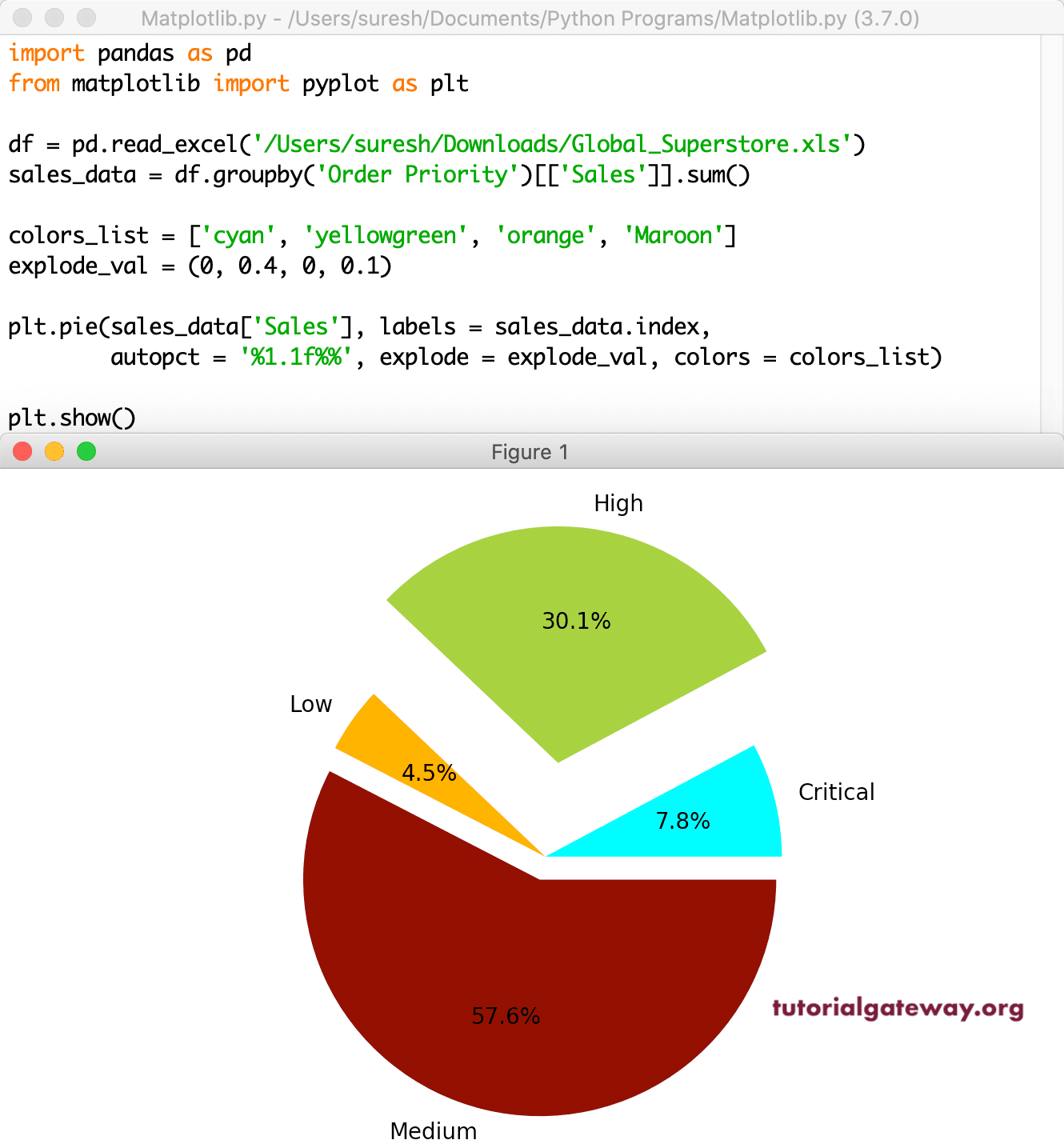
Python matplotlib Pie Chart
How to Combine or Group Pie Charts in Microsoft Excel Combine Pie Chart into a Single Figure. Another reason that you may want to combine the pie charts is so that you can move and resize them as one. Click on the first chart and then hold the Ctrl key as you click on each of the other charts to select them all. Click Format > Group > Group. All pie charts are now combined as one figure.
Combine pie and xy scatter charts - Advanced Excel Charting Example
How to add data labels from different column in an Excel chart? Please do as follows: 1. Right click the data series in the chart, and select Add Data Labels > Add Data Labels from the context menu to add data labels. 2. Right click the data series, and select Format Data Labels from the context menu. 3.
Post a Comment for "44 multiple data labels excel pie chart"