40 format data labels excel 2016

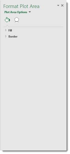
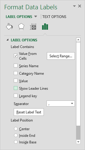
Creating a chart with dynamic labels - Microsoft Excel 2016 1. Right-click on the chart and in the popup menu, select Add Data Labels and again Add Data Labels : 2. Do one of the following: For all labels: on the Format Data Labels pane, in the Label Options, in the Label Contains group, check Value From Cells and then choose cells: For the specific label: double-click on the label value, in the popup ... Format elements of a chart - Microsoft Support Change format of chart elements by using the Format task pane or the ribbon. You can format the chart area, plot area, data series axes, titles, data labels ...

Format Data Labels Vertically using Pareto in Excel 2016 Re: Format Data Labels Vertically using Pareto in Excel 2016. Try this: Right-click on one of the data labels > Format Data Labels > Size & Properties > Alignment > Text direction: Stacked. Register To Reply. 10-03-2017, 01:19 PM #3. 1gambit. Registered User.

Format data labels excel 2016

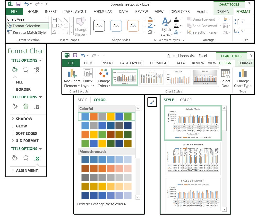
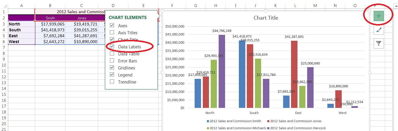
How to Add Total Data Labels to the Excel Stacked Bar Chart Apr 03, 2013 · Step 4: Right click your new line chart and select “Add Data Labels” Step 5: Right click your new data labels and format them so that their label position is “Above”; also make the labels bold and increase the font size. Step 6: Right click the line, select “Format Data Series”; in the Line Color menu, select “No line” How to Customize Chart Elements in Excel 2016 - dummies To add data labels to your selected chart and position them, click the Chart Elements button next to the chart and then select the Data Labels check box before you select one of the following options on its continuation menu: Center to position the data labels in the middle of each data point. Inside End to position the data labels inside each ... Prepare your Excel data source for a Word mail merge In your Excel data source that you'll use for a mailing list in a Word mail merge, make sure you format columns of numeric data correctly. Format a column with numbers, for example, to match a specific category such as currency. If you choose percentage as a category, be aware that the percentage format will multiply the cell value by 100.

Format data labels excel 2016. How to hide zero data labels in chart in Excel? - ExtendOffice 1. Right click at one of the data labels, and select Format Data Labels from the context menu. See screenshot: 2. In the Format Data Labels dialog, Click Number in left pane, then select Custom from the Category list box, and type #"" into the Format Code text box, and click Add button to add it to Type list box. See screenshot: 3. Change Horizontal Axis Values in Excel 2016 - AbsentData 1. Select the Chart that you have created and navigate to the Axis you want to change. 2. Right-click the axis you want to change and navigate to Select Data and the Select Data Source window will pop up, click Edit 3. The Edit Series window will open up, then you can select a series of data that you would like to change. 4. Click Ok How to Format Excel Pivot Table - Contextures Excel Tips May 23, 2022 · Copy a Custom Style in Excel 2016 or Later. In Excel 2016, the custom pivot table style is not copied, if you use the above technique to copy and paste a pivot table. I found a different way to copy the custom style, and this method also works in Excel 2013. In Excel 2016, follow these steps to copy a custom style into a different workbook: Change the format of data labels in a chart To get there, after adding your data labels, select the data label to format, and then click Chart Elements > Data Labels > More Options. To go to the appropriate area, click one of the four icons ( Fill & Line , Effects , Size & Properties ( Layout & Properties in Outlook or Word), or Label Options ) shown here.

Format Data Labels in Excel- Instructions - TeachUcomp, Inc. Nov 14, 2019 · Alternatively, you can right-click the desired set of data labels to format within the chart. Then select the “Format Data Labels…” command from the pop-up menu that appears to format data labels in Excel. Using either method then displays the “Format Data Labels” task pane at the right side of the screen. Format Data Labels in Excel ... Excel 2016 Tutorial Formatting Data Labels Microsoft Training ... - YouTube FREE Course! Click: about Formatting Data Labels in Microsoft Excel at . A clip from Mastering Excel M... How to add or move data labels in Excel chart? - ExtendOffice 2. Then click the Chart Elements, and check Data Labels, then you can click the arrow to choose an option about the data labels in the sub menu. See screenshot: In Excel 2010 or 2007. 1. click on the chart to show the Layout tab in the Chart Tools group. See screenshot: 2. Then click Data Labels, and select one type of data labels as you need ... How to Print Labels from Excel - Lifewire Select Mailings > Write & Insert Fields > Update Labels . Once you have the Excel spreadsheet and the Word document set up, you can merge the information and print your labels. Click Finish & Merge in the Finish group on the Mailings tab. Click Edit Individual Documents to preview how your printed labels will appear. Select All > OK .

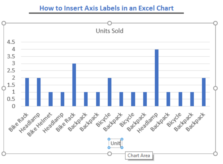
Edit titles or data labels in a chart - Microsoft Support Edit the contents of a title or data label on the chart · Click in the title box, and then select the text that you want to format. · Right-click inside the text ... How to Create Mailing Labels in Excel - Excelchat Step 1 - Prepare Address list for making labels in Excel First, we will enter the headings for our list in the manner as seen below. First Name Last Name Street Address City State ZIP Code Figure 2 - Headers for mail merge Tip: Rather than create a single name column, split into small pieces for title, first name, middle name, last name. How to Change Excel Chart Data Labels to Custom Values? May 05, 2010 · Now, click on any data label. This will select “all” data labels. Now click once again. At this point excel will select only one data label. Go to Formula bar, press = and point to the cell where the data label for that chart data point is defined. Repeat the process for all other data labels, one after another. See the screencast. Excel 2016: How to Format Data and Cells - UniversalClass.com To do this, go to the Format Cells dialogue box again, and click Custom n the category column. In the Type list, select the format that you want to customize. As you can see in the snapshot above, we chose the currency format. Now go to the Type field and customize the format by entering the format you want to use. Click OK when you're finished.

Excel 2016: Creating Charts and Diagrams | UniversalClass

How to Customize Your Excel Pivot Chart Data Labels - dummies To remove the labels, select the None command. If you want to specify what Excel should use for the data label, choose the More Data Labels Options command from the Data Labels menu. Excel displays the Format Data Labels pane. Check the box that corresponds to the bit of pivot table or Excel table information that you want to use as the label.

6 Ghs Safety Data Sheet Template | FabTemplatez

Conditional formatting of chart axes - Microsoft Excel 2016 To change the format of the label on the Excel 2016 chart axis, do the following: 1. Right-click in the axis and choose Format Axis... in the popup menu: 2. On the Format Axis task pane, in the Number group, select Custom category and then change the field Format Code and click the Add button: If you need a unique representation for positive ...

How To Change X Axis Labels In Excel

Add or remove data labels in a chart - support.microsoft.com Click Label Options and under Label Contains, pick the options you want. Use cell values as data labels You can use cell values as data labels for your chart. Right-click the data series or data label to display more data for, and then click Format Data Labels. Click Label Options and under Label Contains, select the Values From Cells checkbox.

Excel charts: Mastering pie charts, bar charts and more - Excel, Office 2013, Office 2016 - PC World

Excel 2016 VBA Display every nth Data Label on Chart Click on the bar you want to labeled twice before Add Data Labels. Click on the label, then right click and select Format Data Labels. Check the Category Name and uncheck Value. A little research before asking can save you a lot of time. Share answered Nov 7, 2017 at 13:15 user8753746 Add a comment

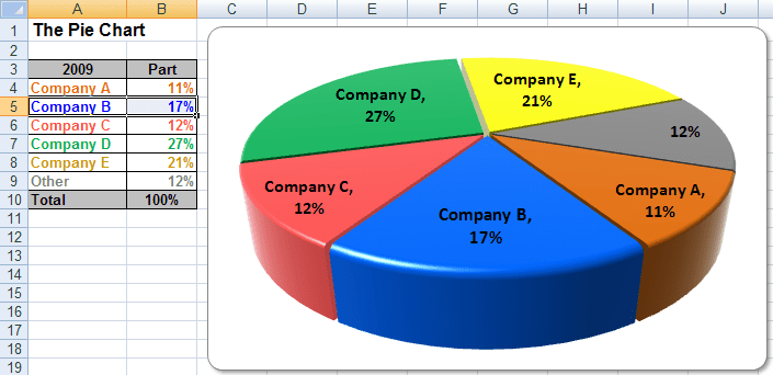
Excel 3-D Pie Charts

Move data labels - support.microsoft.com Click any data label once to select all of them, or double-click a specific data label you want to move. Right-click the selection > Chart Elements > Data Labels arrow, and select the placement option you want. Different options are available for different chart types.

How To Add Text To Bar Chart In Excel - Chart Walls

Create Dynamic Chart Data Labels with Slicers - Excel Campus Feb 10, 2016 · Step 3: Use the TEXT Function to Format the Labels. Typically a chart will display data labels based on the underlying source data for the chart. In Excel 2013 a new feature called “Value from Cells” was introduced. This feature allows us to specify the a range that we want to use for the labels.

35 Label Excel - Labels 2021

3D maps excel 2016 add data labels Re: 3D maps excel 2016 add data labels. I don't think there are data labels equivalent to that in a standard chart. The bars do have a detailed tool tip but that required the map to be interactive and not a snapped picture. You could add annotation to each point. Select a stack and right click to Add annotation. Cheers.

30 What Is A Data Label In Excel - Labels Database 2020

Format Data Label: Label Position - Microsoft Community Hi, I'm using MS Excel 2016 and trying to format data label position to be on top of the bar chart. However, I can't seem to find the 'Label ...

Format Data Labels in Excel- Instructions | Microsoft excel, Microsoft, Bar chart

Excel Charts: Creating Custom Data Labels - YouTube In this video I'll show you how to add data labels to a chart in Excel and then change the range that the data labels are linked to. This video covers both W...

Custom Chart Labels Using Excel 2013 | MyExcelOnline

excel - Change format of all data labels of a single series at once ... A workaround (found prior to #1): A very poor solution, but which possibly saves quite a few keystrokes/mouse clicks in many cases. Select the whole chart, and change the font size in the ribbon. It will change all text. Then recover the font size of all other text but the data labels.

Format Data Labels in Excel- Instructions - TeachUcomp, Inc.

Excel 2016: "Value from Cells" box under Format Data Labels Missing 1. The screenshot about the issue. 2. The Office version screenshot via File > Account > Product Information. We will check whether the issue can be reproduced in a specific version. To protect your privacy, please help us mask email address like below: Thanks, Rena ----------------------- * Beware of scammers posting fake support numbers here.

Download Format Daftar Hadir Bulanan Siswa

Excel 2010: How to format ALL data point labels SIMULTANEOUSLY If you want to format all data labels for more than one series, here is one example of a VBA solution: Code: Sub x () Dim objSeries As Series With ActiveChart For Each objSeries In .SeriesCollection With objSeries.Format.Line .Transparency = 0 .Weight = 0.75 .ForeColor.RGB = 0 End With Next End With End Sub. B.

How to set and format data labels for Excel charts in C#

Edit titles or data labels in a chart - support.microsoft.com The first click selects the data labels for the whole data series, and the second click selects the individual data label. Right-click the data label, and then click Format Data Label or Format Data Labels. Click Label Options if it's not selected, and then select the Reset Label Text check box. Top of Page

30 How To Add Label To Excel Chart - Labels Database 2020

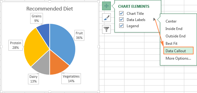
How to create Custom Data Labels in Excel Charts Right click on any data label and choose the callout shape from Change Data Label Shapes option. Now adjust each data label as required to avoid overlap. Put solid fill color in the labels Finally, click on the chart (to deselect the currently selected label) and then click on a data label again (to select all data labels).

Microsoft Tips with Temo!: How to Add Data Labels to an Excel 2010 Chart

Prepare your Excel data source for a Word mail merge In your Excel data source that you'll use for a mailing list in a Word mail merge, make sure you format columns of numeric data correctly. Format a column with numbers, for example, to match a specific category such as currency. If you choose percentage as a category, be aware that the percentage format will multiply the cell value by 100.

How to make a pie chart in Excel

How to Customize Chart Elements in Excel 2016 - dummies To add data labels to your selected chart and position them, click the Chart Elements button next to the chart and then select the Data Labels check box before you select one of the following options on its continuation menu: Center to position the data labels in the middle of each data point. Inside End to position the data labels inside each ...

35 How To Label In Excel - Labels Database 2020

How to Add Total Data Labels to the Excel Stacked Bar Chart Apr 03, 2013 · Step 4: Right click your new line chart and select “Add Data Labels” Step 5: Right click your new data labels and format them so that their label position is “Above”; also make the labels bold and increase the font size. Step 6: Right click the line, select “Format Data Series”; in the Line Color menu, select “No line”

Share :